Primary author: Lily Fu

Applying machine learning algorithms to your business process can be quite beneficial: whether it is to predict incoming workloads to better allocate internal and external resources, or to segment customer groups to personalize marketing campaigns, machine learning is the key to success. Nowadays, it is very easy to train a model with the help of various mature commercial or open source AI platforms. However, when it comes to model performance in the business world, few of them could survive the real test of production. How to develop a model that is production worthy remains the main challenge.

To solve this challenge, you need to understand why your model does not perform as expected and how to correct it. In this post, I would like to introduce the theoretical reason behind the poor performance of your model and show an important technique you could apply to overcome it.

Why does my trained model perform poorly in the real world?

– The nature of overfitting

When we talk about machine learning or deep learning, what we are really talking about is math or statistics. Don’t panic when you see these words. For now, we’ll focus on the first. You don’t need to understand any math equations to follow this part of the article, you only need to treat them as ‘blur’ and believe that this blur can solve it. So keep your eyes peeled.

Back to the topic, ‘blur’ solves everything. This was said by Taylor, not Taylor Swift, but Brook Taylor at 1715. According to Taylor’s theorem, any complex phenomenon/problem could be summarized by Taylor expansion. When training a model your machine is learning the ‘blur’ behind your data. And the more accurate the ‘blur’ is, the more complex your model tends to become. That’s when overfitting happens. By nature, your machine wants to capture all aspects of your data and summarize it with ‘blur’ as accurately as possible.

Overfitting is something you want to avoid if you want your model to be usable. Because The ‘blur’ summarizes signals in your training data. You can prepare your training data to be as extensive as possible, although, it is hard to say that your training data has captured all circumstances of the real world, called generalization. So even if your ‘blur’ is 100 percent accurate for your training set, well, especially then, the over complicated ‘blur’ would not perform well when applying it to the real world; i.e. it does not generalize.

So how do I correct it?

– Regularization to the rescue

To train a good machine learning model that performs well in the real world, regularization is an important technique. It discourages complex models and attempts to limit the overfitting problem of your model. The idea of regularization revolves around modifying the loss function in machine learning.

More specifically, it shrinks the coefficient estimate (weights) of your loss function towards zero. Here, I am going to introduce the ‘blur’ behind two types of regularizations in a simple manner. Continue for some mathematical sensemaking, or skip and remember that everything can be solved by ‘blur’.

Mathematically, regularization adds restrictions to the loss function. By shrinking the weights of your loss function, it makes the curve fitting of your model smoother, and less likely driven by extreme data points. If you knew a little bit of derivatives, you could imagine that the smaller a derivative is, the less angled the trend line would be, hence the smoother the curve. We want the curve fitting of the model to be as smooth as possible because it represents a model that doesn’t overfit the training data.

To set up restrictions to your weights, there are two common ways in math — the L1 (lasso) regularization and the L2 (Ridge) regularization.

L1 regularization

L1 regularization modifies your weights by adding the L1 norm of the vector. It penalizes the sum of the absolute value of weights. I find the following figure to be very helpful in understanding how it works.

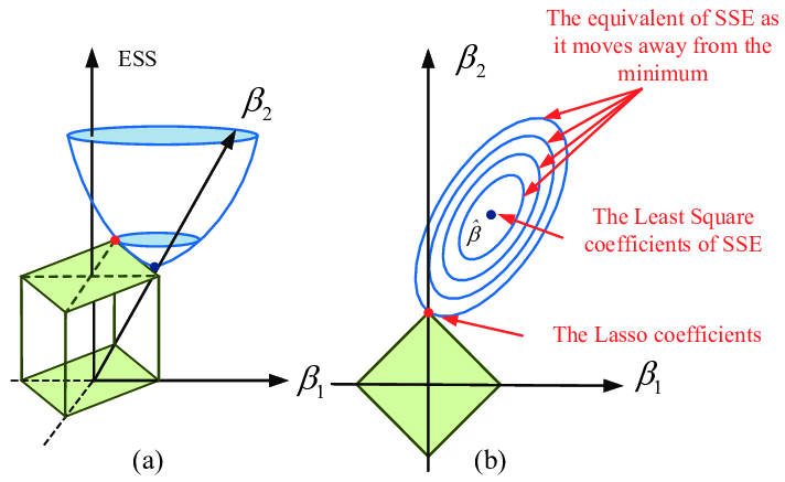
The loss function is plotted at the left, and the regularization term is plotted at the right. To solve the equation, we make them meet each other in the plot. Here you can see that if there are irrelevant input features, Lasso is likely to make their weights 0, which also makes Lasso biased towards providing sparse solutions in general, leaving us with models that are simple and interpretable.

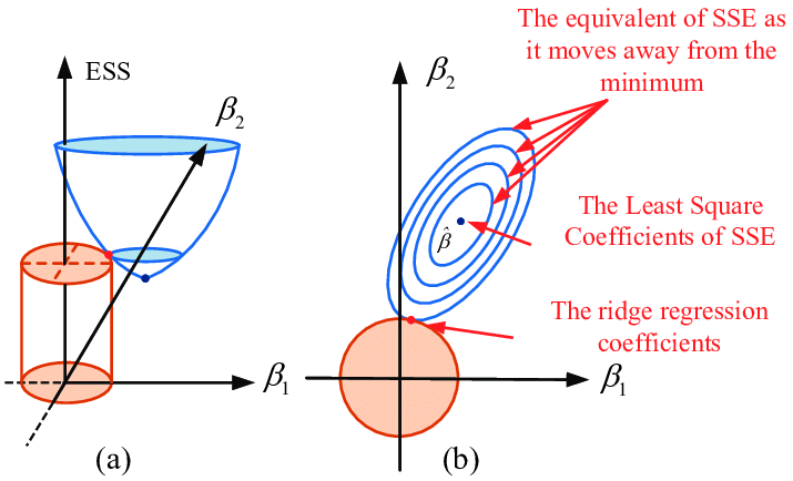
L2 regularization

L2 regularization uses the L2 norm of the vector. It adds “squared magnitude” of coefficient as penalty term to the loss function. Similarly, the following figure illustrates how this type of regularization works in terms of minimizing weights. Different from L1 regularization that forces certain weights of features to be 0, L2 just makes all weights small. Although it doesn’t have the feature selection capability by nature, L2 gives better prediction when output variable is a function of all input features and it is also able to learn complex data patterns.

Visualize the effect of regularization

Here, I provided a code example to visualize the effect of L2 regularization. We are going to train a neural network to generate an overfitted model for binary classification, using the make moons data set from sklearn. To make sure the model is overfitting, we only use 30 data points for training, but we make a layer with 500 nodes, and take 4000 epochs to train this model.

#make example data set

X, y = make_moons(n_samples=100, noise=0.2, random_state=1)
df=DataFrame(dict(x=X[:,0], y=X[:,1], label=y))
colors={0:’green’, 1:’red’}
fig, ax=pyplot.subplots()
grouped=df.groupby(‘label’)
for key, group in grouped:
group.plot(ax=ax, kind=’scatter’, x=’x’, y=’y’, label=key, color=colors[key])
pyplot.show()

#overfitting

n_train=30
trainX, testX=X[:n_train, :], X[n_train:, :]trainy, testy=y[:n_train], y[n_train:]model=Sequential()
model.add(Dense(500, input_dim=2, activation=’relu’))
model.add(Dense(1, activation=’sigmoid’))
model.compile(loss=’binary_crossentropy’, optimizer=’adam’, metrics=[‘accuracy’])

history = model.fit(trainX, trainy, validation_data=(testX, testy),epochs=4000, verbose=0)

_, train_acc=model.evaluate(trainX, trainy, verbose=0)
_, test_acc=model.evaluate(testX, testy, verbose=0)
print(‘Train: %.3f, Test: %.3f’ % (train_acc, test_acc))

Train: 1.00, Test: 0.914

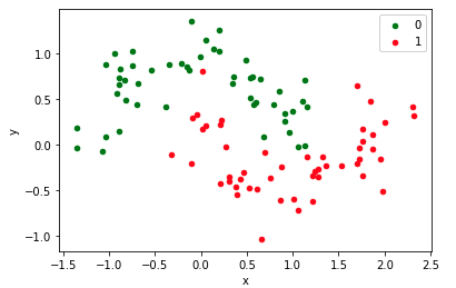
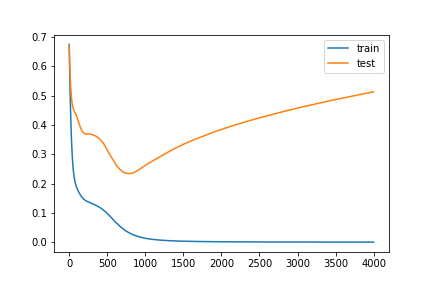
As illustrated by the figure and code, test performance became worse as the model overfits itself. However, simply by adding L2 regularization in your code, test performance remains relatively stable, indicating that overfitting of the model is limited.

#add l2 regularizationmodel_l2=Sequential()

model_l2.add(Dense(500, input_dim=2, activation=’relu’, kernel_regularizer=l2(0.001)))
model_l2.add(Dense(1, activation=’sigmoid’))
model_l2.compile(loss=’binary_crossentropy’, optimizer=’adam’, metrics=[‘accuracy’])
history_12=model_l2.fit(trainX, trainy, validation_data=(testX, testy),epochs=4000, verbose=0)

Train: 1.00, Test: 0.943

Summary

In this article, we brought up a theoretical challenge you must face when bringing your ML models to production — the overfitting nature of machine learning. And we introduced a well-established technique — regularization — to overcome this challenge. There are other techniques such as early stopping and dilution to prevent overfitting.

Productionizing machine learning models can bring huge beneficial effects to your business. Well, one must admit that it is tricky to apply ML models in business production. There are other challenges remaining, such as the scalability of your code, managing the development cycle, and building a core team. We will cover these topics in later articles.

Author Profile

Lily Fu

Data scientist/engineer at Sogeti, PhD in Neuroscience